

TRACE Commercial: Adapting Wall Recovery to Commercial Floor Plans
1. Introduction
A takeoff starts with wall length. Stud counts, plates, sheathing, insulation, gypsum board and several finishes are derived directly from recovered wall geometry, so a wall model that is wrong in a systematic way propagates that error into every downstream quantity [2]. TRACE recovers walls from the vector primitives already present in a construction PDF [1]. Deterministic geometry proposes candidate wall lines; learned models decide which candidates are walls, where they end, which of them describe the same physical wall, and which side of the building each run faces.
TRACE was developed on residential construction drawings, and its learned stages, the pixel wall model RoomNet and the line picker QuantityNet, were trained on house plans [1]. On those populations it performs well. Commercial drawings differ in ways the house corpus rarely shows: poché-filled masonry, double-line demising and rated walls, dense casework, column grids, keynote tags, hatch fields, and scales from 1/8 in. to 3/8 in. per foot. In production these sheets failed in three visible ways: long runs traced as fragments, whole walls dropped, and interior partitions labelled exterior.
Most floor-plan work starts from raster images and predicts walls, rooms or junctions as pixels or graphs [6, 7]; blueprint vectorization has also been attempted directly on high-resolution drawings [8]. TRACE instead keeps the PDF's own vector primitives and uses learning only to verify them [1]. Adapting a trained network to a small new domain by fine-tuning is standard practice [9], with the known risk of forgetting the source domain [10]; both effects appear below.
This paper reports the first adaptation of TRACE to commercial plans. The contributions are:
- a commercial reference set with checked scales and exterior, interior and opening classes, with evaluation sheets held out by project;
- a fine-tuning recipe for RoomNet with ablations over commercial data volume, class weight, initialization, scale augmentation and seed;
- a full-pipeline evaluation on held-out sheets that runs the production client and runtime code in a library environment matched to the production worker; and
- a line picker retrained on production-path inputs and scored end to end, with a negative result that localizes the remaining error.
2. The TRACE model
The name describes the method. TRACE never draws walls from pixels. It first turns a sheet into tokens: each token is one candidate wall line recovered from the PDF's own vector CAD elements, such as parallel face pairs, filled wall bodies, stroke envelopes and bounded continuations. A token then receives a learned representation, and every output coordinate is inherited from a token rather than from a raster (Fig. 1).
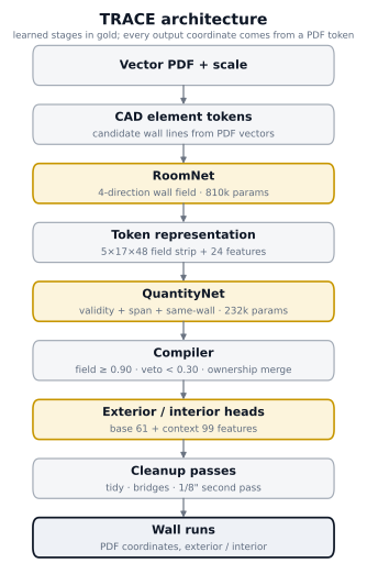
RoomNet is a five-level U-Net [3] with encoder widths 12–24–48–96–128 and 810,096 parameters. It reads the sheet rendered in grayscale at 4 pixels per foot and emits four wall-probability channels for walls near 0°, 45°, 90° and 135°.
Token representation. For each token, a 5×17×48 strip is sampled along it at 8 px/ft: ink darkness plus the four RoomNet channels rotated into the token's frame, 2 ft wide and 48 samples long. Twenty-four numeric features add length, width, field statistics, face-pair support and extraction path.
QuantityNet, the line picker (231,588 parameters), maps the representation to a validity logit and trimmed span endpoints. A pair head receives two token embeddings and eight pair features and predicts whether overlapping parallel tokens are the same physical wall.
Compiler and heads. The compiler keeps RoomNet intervals at or above 0.90, vetoes tokens the line picker scores below 0.30, and merges tokens into runs by ownership. Two small MLP heads then label each run: a base head on 61 geometric and field features and a residual context head that adds 38 room-context features. Cleanup passes (tidy, room bridges, outline snap and a 1.5× second pass on 1/8 in. sheets) follow.
Because the wall field enters the line picker's strips and the heads' features, a new RoomNet changes the inputs of every later learned stage. This coupling determines the experimental order in Sec. 4.
3. Data
3.1 Commercial reference set
Sheets were drawn from Foreman AI's corpus of nearly 98,000 real engineered plans (about 3.6 million pages), choosing commercial floor plans across building types and drafting styles: clinics, a surgery center, restaurants, office and retail tenant improvements, a bank branch and a winery. Reference walls are centrelines tagged exterior, interior or bearing, with openings represented as spans along the wall line.
Every reference sheet carries a checked drawing scale; a wrong scale silently halves or doubles every quantity measured in feet. The five held-out sheets come from five projects, none shared with any training sheet, and range from 1/8 in. to 1/4 in. per foot and from a winery to a cardiology clinic (Table 1).
3.2 House check
The house models and their evaluation sets are unchanged from Report 1 [1]. The same 20 house development sheets serve as the house check in every experiment, so each result reports both what commercial gained and what houses lost.
| Held-out sheet | Scale | Walls | Open. | Ext. LF | Int. LF | Open. LF |
|---|---|---|---|---|---|---|
| H1 (urgent-care clinic) | 1/8" | 161 | 61 | 481 | 1,182 | 145 |
| H2 (winery) | 1/8" | 312 | 27 | 417 | 382 | 107 |
| H3 (restaurant) | 1/4" | 143 | 15 | 179 | 181 | 70 |
| H4 (angled plan) | 3/16" | 105 | 55 | 452 | 682 | 129 |
| H5 (cardiology clinic) | 3/16" | 347 | 120 | 584 | 1,947 | 277 |
| Total (5 sheets) | 1,068 | 278 | 2,113 | 4,374 | 728 |
4. Method
4.1 RoomNet fine-tuning
The selected recipe initialises RoomNet from its production weights and fine-tunes it on a mix of house and commercial sheets with the production four-direction targets, using AdamW [4] with cosine decay; commercial examples are sampled ten times as often as house examples. Ablations vary the amount of commercial data (progressively larger commercial subsets A, B and C), the commercial sampling weight, initialization from scratch versus production weights, scale augmentation and seed.
4.2 Evaluation
Pixel wall F1 at 1 ft compares RoomNet's thresholded field with the reference masks, counting a pixel as matched within one foot, in the spirit of buffer-based positional accuracy [5]. It isolates the wall model but ignores every later stage.
Full-pipeline wall length. Each held-out sheet runs through the production client and runtime (v16.2.4), with its PDF library and software environment matched package-for-package to the production worker. Reference and traced walls are drawn as one-pixel centrelines at 8 px/ft with openings excluded. With G the reference centrelines, T the traced centrelines, L(·) length and N1(·) the 1-ft neighbourhood:
invented = L(T \ N1(G)).
Exterior/interior accuracy samples every traced wall each half foot and compares each sample within 1 ft of a reference wall with that wall's class, weighted by length.
The production sheet gate refuses two of the five held-out sheets, and the manual box fallback refuses a third because a hatch path crosses the box edge. To measure the models rather than the gate, every held-out run uses a box around the drawing whose redaction keeps every path that reaches it. The box stands in for a gate that accepts commercial plans.
4.3 Line-picker retraining
The production line picker never saw fields from the commercial RoomNet. We therefore retrained it on token features computed by the production runtime's own stages (vector extraction, the 4 px/ft render, the commercial RoomNet field and the QuantityNet input packer), so that training and inference see identical inputs. We compare fine-tuning from the production line picker, which keeps its input normalisation, with training from scratch under the original recipe, sampling commercial tokens with weight 1× or 3×. Both keep the original targets and losses: length-weighted validity cross-entropy, span regression and balanced same-wall cross-entropy.
5. Results
5.1 RoomNet
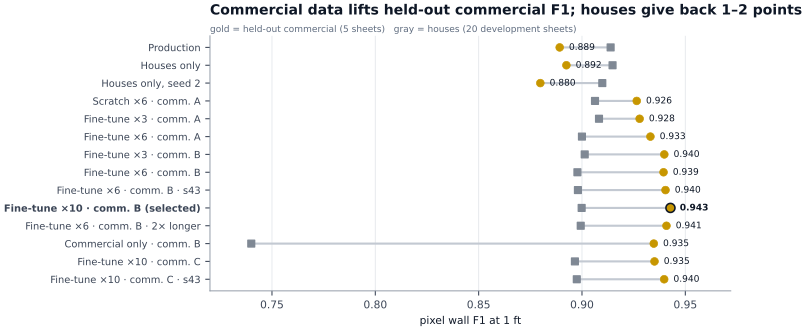
The production model's commercial errors are mostly misses: precision 0.922, recall 0.859. The selected fine-tune holds precision at 0.917 and raises recall to 0.971. Table 2 and Fig. 2 list every run on identical populations.
- Commercial data helps immediately. The smallest commercial subset (A) lifts held-out commercial F1 from about 0.89 to 0.93; houses-only retrains of the same architecture reach 0.880 and 0.892.
- Fine-tuning matches training from scratch with far less compute (0.928 versus 0.926 on subset A) and reaches 0.939–0.943 on subset B.
- More data helps, then saturates. Moving from subset A to B gains about a point; moving from B to the larger subset C gains nothing measurable (0.935 and 0.940 over two seeds versus 0.943).
- Weighting barely matters: commercial ×3, ×6 and ×10 land within 0.004.
- Houses pay a small price. Every mix loses 1–1.7 points on the house set; commercial-only training keeps commercial F1 (0.935) but collapses houses to 0.740, the familiar forgetting of fine-tuned networks [10].
- Scale augmentation hurts: randomly rescaling tiles to imitate 1/8 in. sheets lowered commercial F1 from 0.918 to 0.904 on an earlier, smaller held-out set.
Seed-to-seed spread on the commercial set is about half a point, so smaller differences are not interpreted.
| Run | Training data | Init | Comm. × | Comm. F1 | Houses F1 | External-8 F1 |
|---|---|---|---|---|---|---|
| Production RoomNet | houses (production) | – | – | 0.889 | 0.914 | 0.868 |
| Houses only, retrained | houses | scratch | – | 0.892 | 0.915 | 0.925 |
| Houses only, other seed | houses | scratch | – | 0.880 | 0.910 | 0.891 |
| First commercial mix | houses + comm. A | scratch | ×6 | 0.926 | 0.906 | 0.921 |
| Fine-tune | houses + comm. A | production | ×3 | 0.928 | 0.908 | 0.919 |
| Fine-tune | houses + comm. A | production | ×6 | 0.933 | 0.900 | 0.914 |
| Fine-tune | houses + comm. B | production | ×3 | 0.940 | 0.901 | 0.896 |
| Fine-tune | houses + comm. B | production | ×6 | 0.939 | 0.898 | 0.894 |
| Fine-tune, seed 43 | houses + comm. B | production | ×6 | 0.940 | 0.898 | 0.894 |
| Fine-tune (selected) | houses + comm. B | production | ×10 | 0.943 | 0.900 | 0.894 |
| Fine-tune, 2× longer | houses + comm. B | production | ×6 | 0.941 | 0.899 | 0.904 |
| Commercial only | comm. B only | production | – | 0.935 | 0.740 | 0.786 |
| Fine-tune | houses + comm. C | production | ×10 | 0.935 | 0.897 | 0.882 |
| Fine-tune, seed 43 | houses + comm. C | production | ×10 | 0.940 | 0.897 | 0.894 |
5.2 Full pipeline
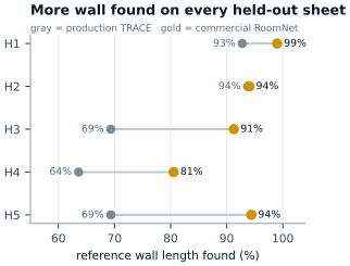
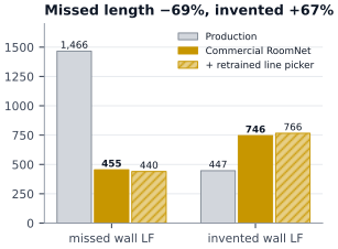
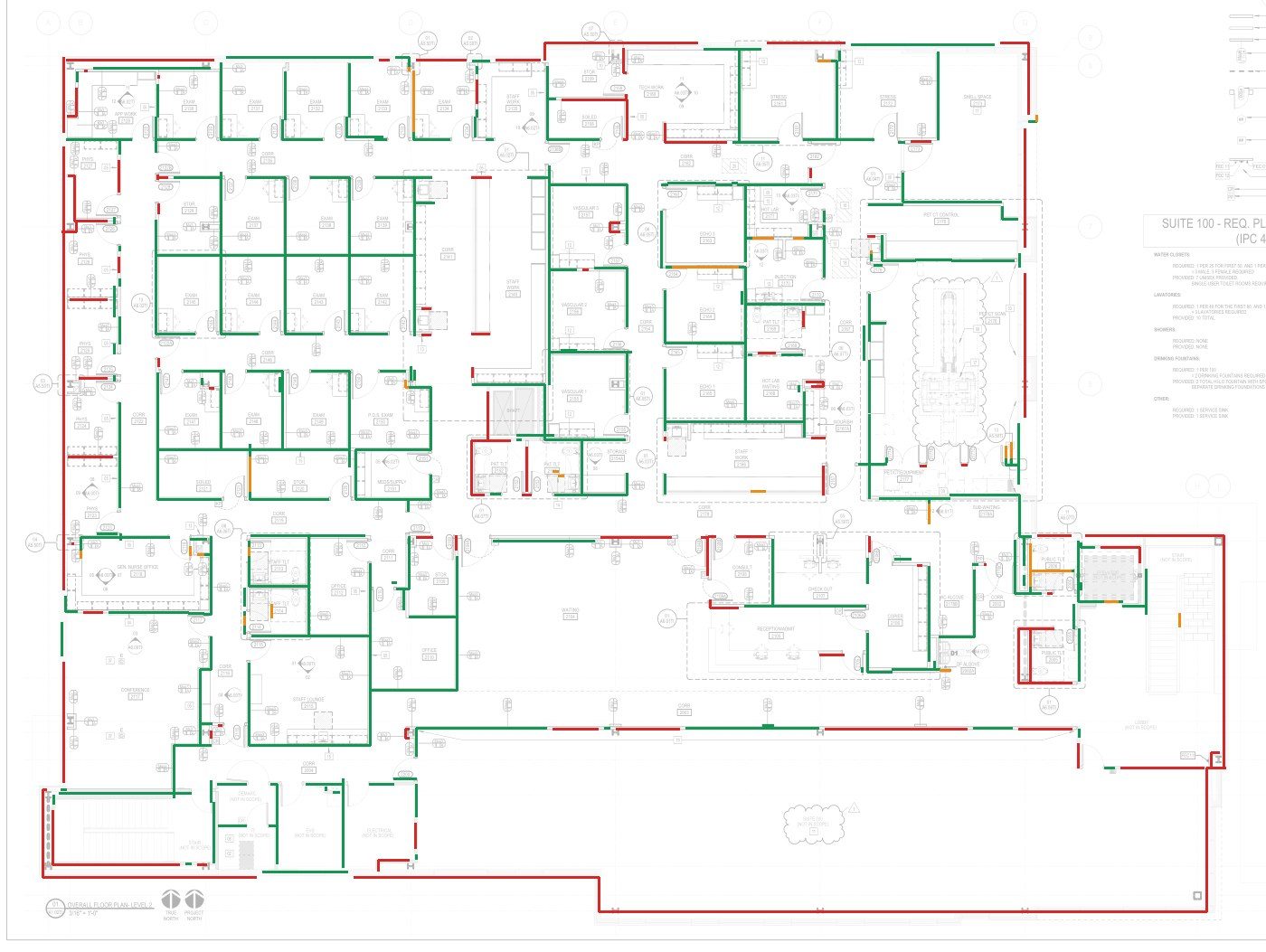
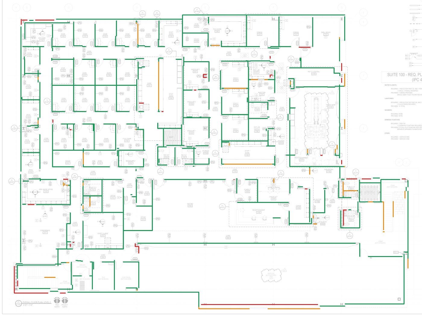
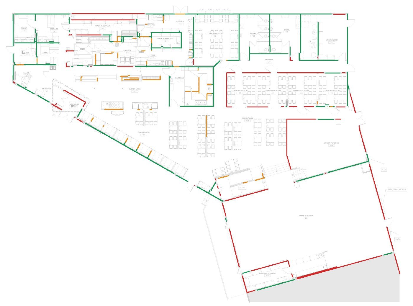
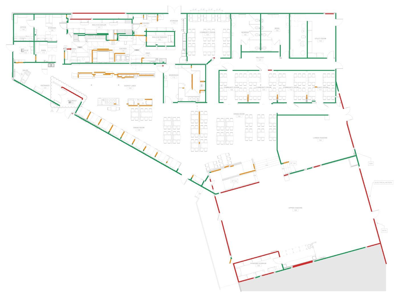
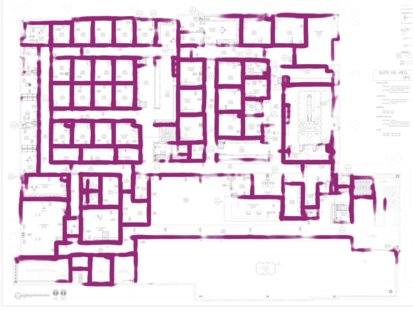
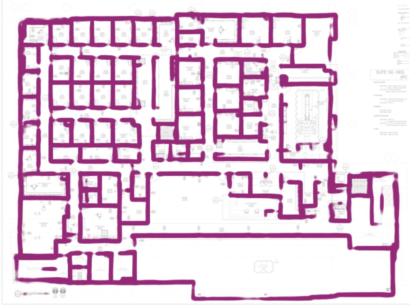
Pixel F1 hides what a takeoff sees. With every stage except RoomNet left at production, found wall length on the held-out sheets rises from 77.4% to 93.0% and missed length falls by 69%, from 1,466 to 455 LF (Table 3, Figs. 3–4). Found length rises on all five sheets; the cardiology clinic moves from 69% to 94%. The cost is invented length, up from 447 to 746 LF, concentrated on casework, fixture outlines, grid stubs and dashed egress paths (Fig. 5). Figure 6 shows the mechanism: the production field fades on thin exterior walls and long corridor walls, and the commercial field does not.
| Held-out sheet | Reference LF | Production: found / missed / invented | Commercial RoomNet: found / missed / invented | + line picker: found / missed / invented |
|---|---|---|---|---|
| H1 (urgent-care clinic) | 1,670 | 1,550 / 121 / 33 | 1,654 / 17 / 50 | 1,653 / 18 / 63 |
| H2 (winery) | 797 | 747 / 50 / 139 | 750 / 48 / 252 | 757 / 40 / 237 |
| H3 (restaurant) | 358 | 248 / 110 / 67 | 326 / 31 / 57 | 327 / 31 / 61 |
| H4 (angled plan) | 1,113 | 708 / 405 / 140 | 896 / 217 / 188 | 901 / 212 / 204 |
| H5 (cardiology clinic) | 2,544 | 1,764 / 780 / 68 | 2,401 / 143 / 199 | 2,404 / 140 / 201 |
| Total | 6,482 | 5,016 (77.4%) / 1,466 / 447 | 6,028 (93.0%) / 455 / 746 | 6,042 (93.2%) / 440 / 766 |
5.3 Exterior and interior
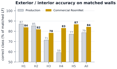
Exterior/interior accuracy also improves overall, from 78.7% to 84.1% (Table 4, Fig. 7). Part of the gain is that the commercial model finds walls the production heads then classify correctly. Per sheet the result is mixed: two sheets (H1, H2) lose three to four points while the other three gain seven to twenty-four. In every column the dominant error is an interior partition called exterior, the natural bias of heads trained only on houses, where long straight walls near the outline are usually exterior.
5.4 Line picker
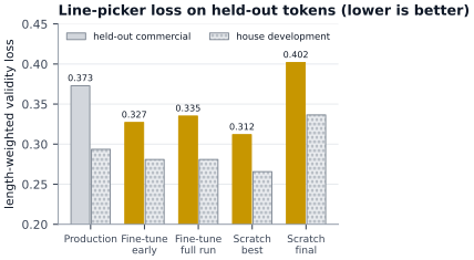
Table 5 and Fig. 8 score each line-picker variant on held-out tokens using the commercial field. Fine-tuning lowers commercial validity loss from 0.373 to 0.327 and keeps two to three points more real wall length at the production veto threshold; house loss also improves. Training from scratch peaks early and then overfits, ending worse than production on both populations by its final checkpoint. The pair head is the weak component on commercial sheets, separating same-wall from different-wall pairs only 60–67% of the time against about 76% on houses. The hard cases are walls within a foot of each other: demising walls, furring and chase walls.
The token-level gain does not carry through. Run end to end, the fine-tuned line picker moves found length from 93.0% to 93.2%, missed length from 455 to 440 LF, invented length from 746 to 766 LF and exterior/interior accuracy from 84.1% to 84.4%, all inside the noise. The retrained model mainly raises its scores on real walls; its veto removes about as much non-wall length as before, and the walls the full pipeline invents pass the veto with either model.
| Held-out sheet | Production: correct (LF compared) | Commercial RoomNet: correct (LF compared) | + line picker: correct (LF compared) |
|---|---|---|---|
| H1 (urgent-care clinic) | 87.1% (1,316) | 83.7% (1,445) | 83.6% (1,417) |
| H2 (winery) | 85.3% (975) | 81.7% (956) | 82.5% (947) |
| H3 (restaurant) | 71.4% (239) | 78.2% (330) | 76.4% (343) |
| H4 (angled plan) | 59.2% (686) | 83.0% (898) | 81.6% (907) |
| H5 (cardiology clinic) | 77.2% (1,627) | 86.6% (2,322) | 87.8% (2,357) |
| All | 78.7% (4,843) | 84.1% (5,951) | 84.4% (5,971) |
| Interior called exterior (LF) | 937 | 755 | 752 |
| Exterior called interior (LF) | 95 | 190 | 181 |
| Line picker | C loss | C kept | C removed | C pair | H loss | H kept | H removed | H pair |
|---|---|---|---|---|---|---|---|---|
| Production line picker (new field) | 0.373 | 91.8% | 83.4% | 0.600 | 0.294 | 93.2% | 87.6% | 0.762 |
| Fine-tune ×3, early checkpoint | 0.327 | 94.2% | 82.0% | 0.641 | 0.281 | 95.3% | 85.5% | 0.773 |
| Fine-tune ×3, full run | 0.335 | 93.7% | 83.0% | 0.622 | 0.281 | 94.5% | 86.1% | 0.755 |
| Fine-tune ×1, full run | 0.335 | 93.6% | 82.6% | 0.625 | 0.281 | 94.3% | 86.8% | 0.761 |
| Fine-tune ×3, higher LR, full run | 0.354 | 93.1% | 83.5% | 0.596 | 0.299 | 93.8% | 86.7% | 0.743 |
| Scratch ×3, best checkpoint | 0.312 | 94.7% | 81.7% | 0.673 | 0.266 | 95.2% | 86.2% | 0.764 |
| Scratch ×3, final checkpoint | 0.402 | 91.4% | 84.1% | 0.595 | 0.337 | 93.0% | 88.5% | 0.745 |
6. Discussion
The central result is that the bottleneck moved. Beyond a modest commercial set the pixel model stopped improving on this test, and the full pipeline now finds 93% of commercial wall length. What remains is invented length and class errors. Because a better line picker did not remove the invented walls, either they are produced by stages it does not gate (cleanup passes, perimeter recovery, the 1/8 in. second pass), or the 0.30 veto is too permissive for commercial sheets. The next measurement should attribute each invented foot to the stage that produced it before any further training.
The house cost argues for two models. Every commercial mix gave back 1–1.7 points on houses, which remain most of the production traffic. The runtime should keep the house bundle and route commercial plans to a commercial bundle; the result cache is keyed on the wall-model file, so the two cannot share results.
Environment parity proved material. An earlier run of this comparison in a development environment with an older PDF library than the production worker showed exterior/interior accuracy falling from 83.3% to 67.1% on three sheets. With the worker's exact library version the same three sheets move from 87.1%, 85.3% and 71.4% to 83.7%, 81.7% and 78.2%. The class features read page text and drawings, and both change with the library version. Every result in this paper uses the matched environment.
7. Limitations and threats to validity
- Small commercial test set. Five held-out sheets from five projects detect effects of several points but cannot rank close variants.
- Selection on the test set. Line-picker checkpoints were chosen on the held-out tokens because five sheets leave no separate validation split; token-level numbers are optimistic.
- Bypassed gate. The held-out runs use a lenient box. Today's production path would refuse two of the five sheets outright.
- One reference convention. The reference set follows a single convention for what counts as a wall (for example, centrelines run through doors), so that convention is also the model's.
- Seed variance. Seed-to-seed spread of about half a point on commercial F1 limits every RoomNet comparison below that size.
8. Reproducibility
The commercial reference set and sheet list, the training and evaluation code, the full-pipeline harness, and the scripts that regenerate every figure and number in this paper are retained by Foreman AI Research, together with checkpoint hashes for every run, including the selected commercial RoomNet. Test runtimes are copies of production runtime v16.2.4 with one model swapped and hash pins rewritten in the copy only. Nothing reported here has shipped; production still runs the house models.
9. Conclusion
A small commercial reference set was enough to adapt TRACE's wall model: on held-out commercial sheets the full pipeline now finds 93.0% of wall length instead of 77.4% and misses 455 LF instead of 1,466. The adaptation costs houses 1–2 pixel-F1 points, so the commercial model should be deployed alongside the house model rather than in place of it. The work also shows where effort should go next. More commercial examples no longer move the wall model, and a retrained line picker does not reduce invented length. The next gains will come from finding which stage admits invented walls, retraining the exterior/interior heads on commercial predictions, and fixing the sheet gate so commercial plans reach the model at all.
Data availability
The plan sheets come from Foreman AI's proprietary corpus and are not redistributed; sheets are identified by neutral IDs. Aggregate results, per-sheet scores and checkpoint hashes are retained by Foreman AI Research.
Competing interests
Kyle Rossignol is the founder of Foreman AI LLC, which develops commercial construction-estimating software incorporating the wall-recovery technology described here. This manuscript reports internal research and should be interpreted with that relationship disclosed.
Funding
The work was conducted as internal research and development by Foreman AI LLC. No external funding was received.
Author contributions
K.R. conceived the project, built the commercial reference set, and directed the experiments. Model training, evaluation and drafting of this manuscript were carried out with Claude (Anthropic), an AI model, under K.R.'s direction.
References
- K. Rossignol, “TRACE Residential: Candidate-Then-Verify Wall Recovery from Vector Construction Drawings,” Foreman AI Research, TRACE Series Report 1, Colorado, USA, Sep. 2026.
- K. Rossignol, “Measurement Practice for Automated Wall Recovery from Architectural Construction Drawings,” Foreman AI Research, Colorado, USA, technical report, Aug. 2026.
- O. Ronneberger, P. Fischer, and T. Brox, “U-Net: Convolutional Networks for Biomedical Image Segmentation,” in Medical Image Computing and Computer-Assisted Intervention (MICCAI), pp. 234–241, 2015.
- I. Loshchilov and F. Hutter, “Decoupled Weight Decay Regularization,” in International Conference on Learning Representations (ICLR), 2019.
- M. F. Goodchild and G. J. Hunter, “A simple positional accuracy measure for linear features,” International Journal of Geographical Information Science, vol. 11, no. 3, pp. 299–306, 1997.
- C. Liu, J. Wu, P. Kohli, and Y. Furukawa, “Raster-To-Vector: Revisiting Floorplan Transformation,” in Proc. IEEE International Conference on Computer Vision (ICCV), pp. 2195–2203, 2017.
- A. Kalervo, J. Ylioinas, M. Häikiö, A. Karhu, and J. Kannala, “CubiCasa5K: A Dataset and an Improved Multi-Task Model for Floorplan Image Analysis,” arXiv:1904.01920, 2019.
- W. Song, M. M. Abyaneh, M. A. A. Shabani, and Y. Furukawa, “Vectorizing Building Blueprints,” in Proc. Asian Conference on Computer Vision (ACCV), pp. 1044–1059, 2022.
- J. Yosinski, J. Clune, Y. Bengio, and H. Lipson, “How transferable are features in deep neural networks?,” in Advances in Neural Information Processing Systems (NeurIPS), pp. 3320–3328, 2014.
- J. Kirkpatrick et al., “Overcoming catastrophic forgetting in neural networks,” Proceedings of the National Academy of Sciences, vol. 114, no. 13, pp. 3521–3526, 2017.